1 Iris 꽃 종류 분류
import pandas as pd
import numpy as np
import matplotlib.pyplot as plt


np.random.seed(2021)
1.1 1. Data
1.1.1 1.1 Data Load
데이터는 sklearn.datasets 의 load_iris 함수를 이용해 받을 수 있습니다.
from sklearn.datasets import load_iris

iris = load_iris()
데이터에서 사용되는 변수는 암술과 수술의 길이와 넓이입니다.
- sepal length (cm)
- sepal width (cm)
- petal length (cm)
- petal width (cm)
iris["feature_names"]

>>>
['sepal length (cm)',
 'sepal width (cm)',
 'petal length (cm)',
 'petal width (cm)']
정답은 iris 꽃의 종류입니다.
iris["target_names"]

>>>
array(['setosa', 'versicolor', 'virginica'], dtype='<U10')
data, target = iris["data"], iris["target"]
1.1.2 1.2 데이터 EDA
pd.DataFrame(data, columns=iris["feature_names"]).describe()
1.1.3 1.3 Data Split
from sklearn.model_selection import train_test_split

train_data, test_data, train_target, test_target = train_test_split(
    data, target, train_size=0.7, random_state=2021, stratify=target
)
print("train data 개수:", len(train_data))
print("train data 개수:", len(test_data))

>>>
train data 개수: 105
train data 개수: 45
1.1.4 1.4 시각화
fig, axes = plt.subplots(nrows=2, ncols=3, figsize=(15,10))

pair_combs = [
    [0, 1], [0, 2], [0, 3], [1, 2], [1, 3], [2, 3]
]
for idx, pair in enumerate(pair_combs):
    x, y = pair
    ax = axes[idx//3, idx%3]
    ax.scatter(
        x=train_data[:, x], y=train_data[:, y], c=train_target, edgecolor='black', s=15
    )
    ax.set_xlabel(iris["feature_names"][x])
    ax.set_ylabel(iris["feature_names"][y])
1.2 2. Decision Tree
from sklearn.tree import DecisionTreeClassifier, plot_tree

gini_tree = DecisionTreeClassifier()
1.2.1 2.1 학습
gini_tree.fit(train_data, train_target)

plt.figure(figsize=(10,10))
plot_tree(gini_tree, feature_names=iris["feature_names"], class_names=iris["target_names"])


[Text(0.4, 0.875, 'petal length (cm) <= 2.5\ngini = 0.667\nsamples = 105\nvalue = [35, 35, 35]\nclass = setosa'),
 Text(0.2, 0.625, 'gini = 0.0\nsamples = 35\nvalue = [35, 0, 0]\nclass = setosa'),
 Text(0.6, 0.625, 'petal width (cm) <= 1.65\ngini = 0.5\nsamples = 70\nvalue = [0, 35, 35]\nclass = versicolor'),
 Text(0.4, 0.375, 'petal length (cm) <= 5.35\ngini = 0.102\nsamples = 37\nvalue = [0, 35, 2]\nclass = versicolor'),
 Text(0.2, 0.125, 'gini = 0.0\nsamples = 35\nvalue = [0, 35, 0]\nclass = versicolor'),
 Text(0.6, 0.125, 'gini = 0.0\nsamples = 2\nvalue = [0, 0, 2]\nclass = virginica'),
 Text(0.8, 0.375, 'gini = 0.0\nsamples = 33\nvalue = [0, 0, 33]\nclass = virginica')]
1.2.2 2.2 Arguments
DecisionTreeClassifier에서 주로 탐색하는 argument들은 다음과 같습니다.
- criterion
- 어떤 정보 이득을 기준으로 데이터를 나눌지 정합니다.
- "gini", "entropy"
- max_depth
- 나무의 최대 깊이를 정해줍니다.
- min_samples_split
- 노드가 나눠질 수 있는 최소 데이터 개수를 정합니다.
1.2.2.1 2.2.1 max_depth
depth_1_tree = DecisionTreeClassifier(max_depth=1)
depth_1_tree.fit(train_data, train_target)

plot_tree(depth_1_tree, feature_names=iris["feature_names"], class_names=iris["target_names"])

>>>
[Text(0.5, 0.75, 'petal length (cm) <= 2.5\ngini = 0.667\nsamples = 105\nvalue = [35, 35, 35]\nclass = setosa'),
 Text(0.25, 0.25, 'gini = 0.0\nsamples = 35\nvalue = [35, 0, 0]\nclass = setosa'),
 Text(0.75, 0.25, 'gini = 0.5\nsamples = 70\nvalue = [0, 35, 35]\nclass = versicolor')]
1.2.2.2 2.2.2 min_samples_split
sample_50_tree = DecisionTreeClassifier(min_samples_split=50)
sample_50_tree.fit(train_data, train_target)

plot_tree(sample_50_tree, feature_names=iris["feature_names"], class_names=iris["target_names"])

>>> [Text(0.4, 0.8333333333333334, 'petal width (cm) <= 0.8\ngini = 0.667\nsamples = 105\nvalue = [35, 35, 35]\nclass = setosa'),
     Text(0.2, 0.5, 'gini = 0.0\nsamples = 35\nvalue = [35, 0, 0]\nclass = setosa'),
     Text(0.6, 0.5, 'petal width (cm) <= 1.65\ngini = 0.5\nsamples = 70\nvalue = [0, 35, 35]\nclass = versicolor'),
     Text(0.4, 0.16666666666666666, 'gini = 0.102\nsamples = 37\nvalue = [0, 35, 2]\nclass = versicolor'),
     Text(0.8, 0.16666666666666666, 'gini = 0.0\nsamples = 33\nvalue = [0, 0, 33]\nclass = virginica')]
1.2.2.3 2.2.3 criterion
entropy_tree = DecisionTreeClassifier(criterion="entropy")
entropy_tree.fit(train_data, train_target)

fig, axes = plt.subplots(nrows=1, ncols=2, figsize=(15, 10))
plot_tree(gini_tree, feature_names=iris["feature_names"], class_names=iris["target_names"], ax=axes[0])
plot_tree(entropy_tree, feature_names=iris["feature_names"], class_names=iris["target_names"], ax=axes[1])
plt.show()
1.2.3 2.3 예측
trees = [
    ("gini tree", gini_tree),
    ("entropy tree", entropy_tree),
    ("depth=1 tree", depth_1_tree),
    ("sample=50 tree" ,sample_50_tree),
]
train_preds = []
test_preds = []
for tree_name, tree in trees:
train_pred = tree.predict(train_data)
test_pred = tree.predict(test_data)
train_preds += [train_pred]
test_preds += [test_pred]train_preds
>>>
[array([0, 2, 0, 0, 0, 2, 0, 2, 1, 1, 2, 1, 0, 2, 1, 1, 1, 2, 2, 2, 2, 1,
2, 0, 2, 0, 2, 1, 0, 2, 2, 1, 1, 0, 1, 0, 1, 2, 0, 0, 2, 2, 0, 0,
2, 2, 2, 0, 0, 1, 1, 1, 1, 2, 1, 0, 1, 0, 2, 2, 0, 2, 0, 0, 1, 0,
0, 2, 2, 1, 2, 2, 2, 0, 0, 1, 1, 1, 0, 1, 0, 2, 0, 2, 2, 1, 1, 2,
1, 0, 1, 1, 0, 0, 2, 1, 1, 0, 2, 0, 1, 0, 1, 1, 1]),
array([0, 2, 0, 0, 0, 2, 0, 2, 1, 1, 2, 1, 0, 2, 1, 1, 1, 2, 2, 2, 2, 1,
2, 0, 2, 0, 2, 1, 0, 2, 2, 1, 1, 0, 1, 0, 1, 2, 0, 0, 2, 2, 0, 0,
2, 2, 2, 0, 0, 1, 1, 1, 1, 2, 1, 0, 1, 0, 2, 2, 0, 2, 0, 0, 1, 0,
0, 2, 2, 1, 2, 2, 2, 0, 0, 1, 1, 1, 0, 1, 0, 2, 0, 2, 2, 1, 1, 2,
1, 0, 1, 1, 0, 0, 2, 1, 1, 0, 2, 0, 1, 0, 1, 1, 1]),
array([0, 1, 0, 0, 0, 1, 0, 1, 1, 1, 1, 1, 0, 1, 1, 1, 1, 1, 1, 1, 1, 1,
1, 0, 1, 0, 1, 1, 0, 1, 1, 1, 1, 0, 1, 0, 1, 1, 0, 0, 1, 1, 0, 0,
1, 1, 1, 0, 0, 1, 1, 1, 1, 1, 1, 0, 1, 0, 1, 1, 0, 1, 0, 0, 1, 0,
0, 1, 1, 1, 1, 1, 1, 0, 0, 1, 1, 1, 0, 1, 0, 1, 0, 1, 1, 1, 1, 1,
1, 0, 1, 1, 0, 0, 1, 1, 1, 0, 1, 0, 1, 0, 1, 1, 1]),
array([0, 2, 0, 0, 0, 2, 0, 2, 1, 1, 2, 1, 0, 2, 1, 1, 1, 2, 2, 2, 2, 1,
2, 0, 1, 0, 2, 1, 0, 2, 2, 1, 1, 0, 1, 0, 1, 1, 0, 0, 2, 2, 0, 0,
2, 2, 2, 0, 0, 1, 1, 1, 1, 2, 1, 0, 1, 0, 2, 2, 0, 2, 0, 0, 1, 0,
0, 2, 2, 1, 2, 2, 2, 0, 0, 1, 1, 1, 0, 1, 0, 2, 0, 2, 2, 1, 1, 2,
1, 0, 1, 1, 0, 0, 2, 1, 1, 0, 2, 0, 1, 0, 1, 1, 1])]
1.2.4 2.3 평가하기
from sklearn.metrics import accuracy_score

for idx, (tree_name, tree) in enumerate(trees):
    train_acc = accuracy_score(train_target, train_preds[idx])
    test_acc =  accuracy_score(test_target, test_preds[idx])
    print(tree_name)
    print("\t", f"train accuracy is {train_acc:.2f}")
    print("\t", f"test accuracy is {test_acc:.2f}")

>>>
    gini tree
         train accuracy is 1.00
         test accuracy is 0.91
    entropy tree
         train accuracy is 1.00
         test accuracy is 0.91
    depth=1 tree
         train accuracy is 0.67
         test accuracy is 0.67
    sample=50 tree
         train accuracy is 0.98
         test accuracy is 0.91
1.2.5 2.4 Feature Importance
iris["feature_names"]

>>> ['sepal length (cm)',
     'sepal width (cm)',
     'petal length (cm)',
     'petal width (cm)']


gini_tree.feature_importances_

>>>
array([0.        , 0.        , 0.05405405, 0.94594595])
gini_feature_importance = pd.Series(gini_tree.feature_importances_, index=iris["feature_names"])

gini_feature_importance
>>>
sepal length (cm)    0.000000
sepal width (cm)     0.000000
petal length (cm)    0.054054
petal width (cm)     0.945946
dtype: float64
gini_feature_importance.plot(kind="barh", title="gini tree feature importance")
sample_50_feature_importance = pd.Series(
    sample_50_tree.feature_importances_,
    index=iris["feature_names"]
)

sample_50_feature_importance.plot(kind="barh", title="sample=50 tree feature importance")
1.3 3. 시각화
def plot_decision_boundary(pair_data, pair_tree, ax):
    x_min, x_max = pair_data[:, 0].min() - 1, pair_data[:, 0].max() + 1
    y_min, y_max = pair_data[:, 1].min() - 1, pair_data[:, 1].max() + 1
    xx, yy = np.meshgrid(np.arange(x_min, x_max, 0.02),
                         np.arange(y_min, y_max, 0.02))

    Z = pair_tree.predict(np.c_[xx.ravel(), yy.ravel()])
    Z = Z.reshape(xx.shape)
    cs = ax.contourf(xx, yy, Z, cmap=plt.cm.RdYlBu)

    # Plot the training points
    for i, color in zip(range(3), "ryb"):
        idx = np.where(train_target == i)
        ax.scatter(pair_data[idx, 0], pair_data[idx, 1], c=color, label=iris["target_names"][i],
                    cmap=plt.cm.RdYlBu, edgecolor='black', s=15)
    return ax
fig, axes = plt.subplots(nrows=2, ncols=3, figsize=(15,10))

pair_combs = [
    [0, 1], [0, 2], [0, 3], [1, 2], [1, 3], [2, 3]
]
for idx, pair in enumerate(pair_combs):
    x, y = pair
    pair_data = train_data[:, pair]
    pair_tree = DecisionTreeClassifier().fit(pair_data, train_target)

    ax = axes[idx//3, idx%3]
    ax = plot_decision_boundary(pair_data, pair_tree, ax)
    ax.set_xlabel(iris["feature_names"][x])
    ax.set_ylabel(iris["feature_names"][y])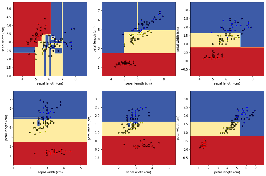
'Machine Learning > 머신러닝 온라인 강의' 카테고리의 다른 글
| CH04_10. Ensemble & Random Forest (0) | 2022.10.10 |
|---|---|
| CH04_07. Iris 꽃 종류 분류 (multiclass,Logistic Regression) (0) | 2022.10.10 |
| CH04_04. Decision Tree Regression 실습 (Python) (0) | 2022.10.10 |
| CH04_02. Decision Tree Classification 실습 (Python) (0) | 2022.10.10 |
| CH04_01. Decision Tree (0) | 2022.10.10 |


