1 모듈 및 데이터 로딩
import pandas as pd
import numpy as np
import matplotlib.pyplot as plt
import seaborn as sns

# 워닝 무시
import warnings
warnings.filterwarnings('ignore')
data = pd.read_csv('smartphone.csv')
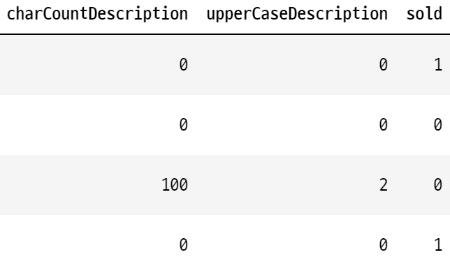
2 데이터(ebay ecommerce) 특성 확인하기
print(data.shape)
data.head(20)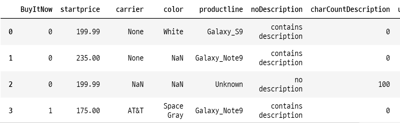
머신러닝 : 지도 학습
<종속변수> -> 예측하고 싶은 것
sold : 판매 여부(1은 판매됨, 0은 판매 안 됨)
<독립변수(피쳐) 후보> -> 기존 주어진 데이터
BuyItNow : 경매없이 바로구매 옵션
startprice : 시작 가격
carrier : 미국 통신사
color : 디바이스 컬러
productline : 모델명
noDescription : 아이템 상세페이지 설명 여부
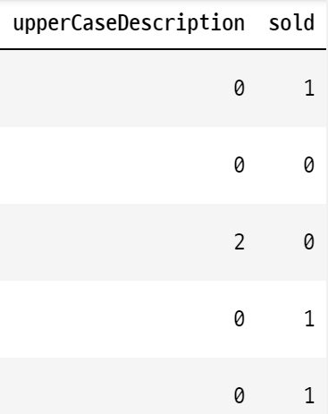
charCountDescription : 글자 길이
upperCaseDescription : 대문자 수(=문장 수)
data.info()

>>>
<class 'pandas.core.frame.DataFrame'>
RangeIndex: 1485 entries, 0 to 1484
Data columns (total 9 columns):
 #   Column                Non-Null Count  Dtype
---  ------                --------------  -----
 0   BuyItNow              1485 non-null   int64
 1   startprice            1485 non-null   float64
 2   carrier               1179 non-null   object
 3   color                 892 non-null    object
 4   productline           1485 non-null   object
 5   noDescription         1485 non-null   object
 6   charCountDescription  1485 non-null   int64
 7   upperCaseDescription  1485 non-null   int64
 8   sold                  1485 non-null   int64
dtypes: float64(1), int64(4), object(4)
memory usage: 104.5+ KB
data.describe()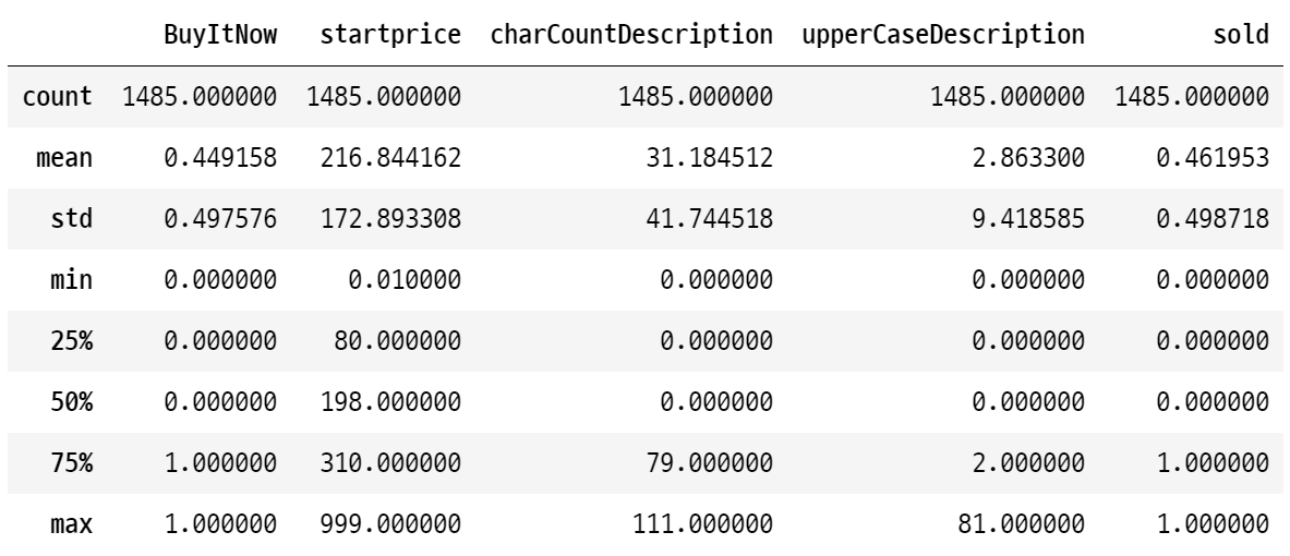
2.1 시각화
# distplot
sns.distplot(data['startprice']);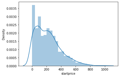
sns.distplot(data['charCountDescription']);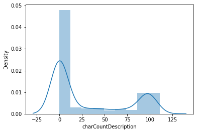
# boxplot
plt.figure(figsize=(20, 10))
sns.boxplot(x='productline', y='startprice', data = data);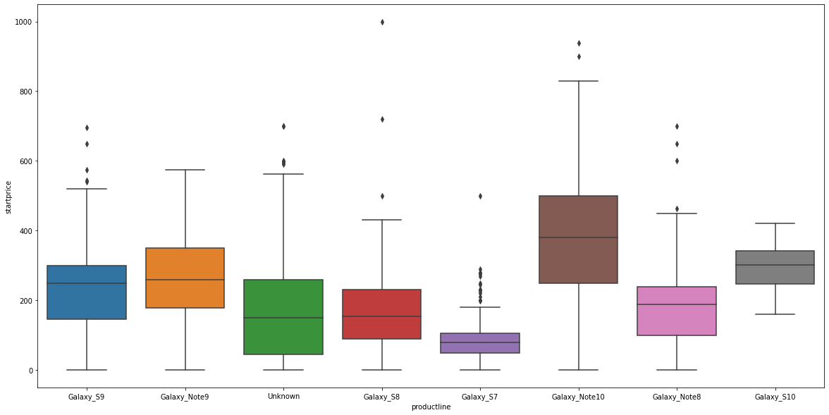
<박스플랏 해석>
@ 박스 : (밑에서부터) 25%/ 50%/ 75%
@ 아래/위 라인
- 아래 라인 : 75% + 1.5IQR
- 위에 라인 : 25% - 1.5IQR
IQR이란, Interquartile range의 약자로써 Q3 - Q1를 의미한다.
# Q3 - Q1: 사분위수의 상위 75% 지점의 값과 하위 25% 지점의 값 차이
@ 위 라인 이상의 값들 : 이상치(outlier)
3 Missing Value 확인 및 처리
data.isna().sum() / len(data)

>>>
BuyItNow                0.000000
startprice              0.000000
carrier                 0.206061
color                   0.399327
productline             0.000000
noDescription           0.000000
charCountDescription    0.000000
upperCaseDescription    0.000000
sold                    0.000000
dtype: float64
data.head(20)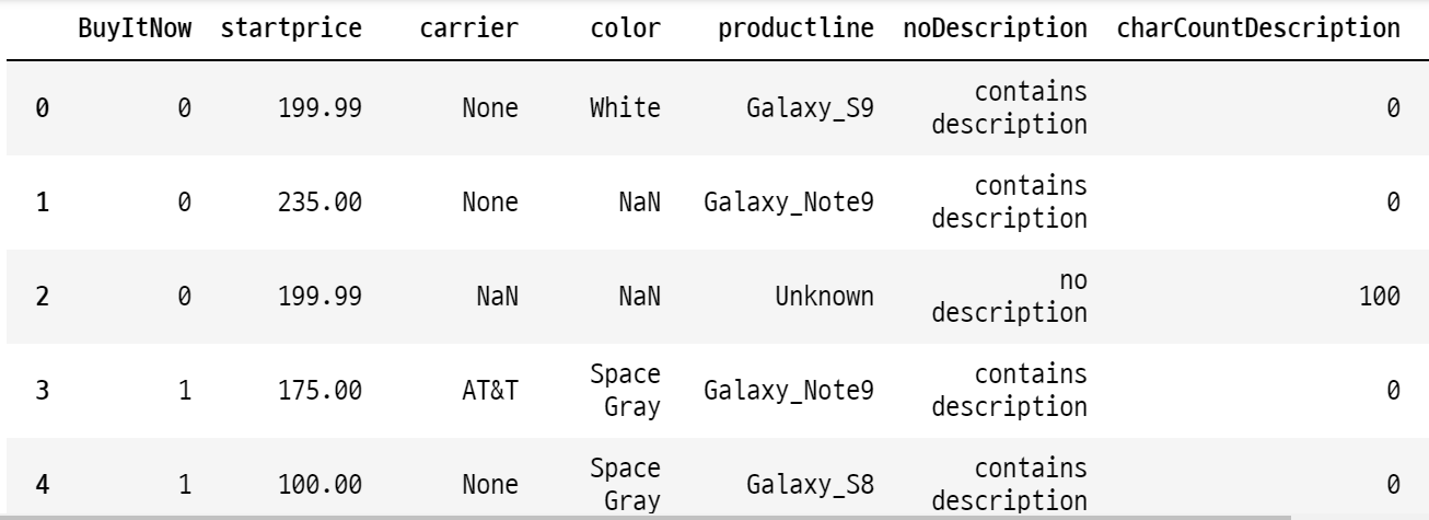
<텍스트 missing value 처리>
@ carrier(통신사)
- carrier는 missing value 채워서 사용하면 될듯
- None은 텍스트 'None'이 들어있는 것
-> None : 자급제 폰
- NaN은 아예 아무것도 없는 것
-> 통신사 정보가 없는 것
-> 'Unknown' 값으로 변경 처리
@ color
- color도 missing value 채워서 사용
data['carrier'].value_counts()

>>>
None               863
Unknown            306
AT&T               177
Verizon             87
Sprint/T-Mobile     52
Name: carrier, dtype: int64
4 카테고리 변수 처리
data.info()

>>>
<class 'pandas.core.frame.DataFrame'>
RangeIndex: 1485 entries, 0 to 1484
Data columns (total 9 columns):
 #   Column                Non-Null Count  Dtype
---  ------                --------------  -----
 0   BuyItNow              1485 non-null   int64
 1   startprice            1485 non-null   float64
 2   carrier               1485 non-null   object
 3   color                 1485 non-null   object
 4   productline           1485 non-null   object
 5   noDescription         1485 non-null   object
 6   charCountDescription  1485 non-null   int64
 7   upperCaseDescription  1485 non-null   int64
 8   sold                  1485 non-null   int64
dtypes: float64(1), int64(4), object(4)
memory usage: 104.5+ KB
>>>
carrier          5
color            8
productline      8
noDescription    2
dtype: int64
data['carrier'].value_counts()
>>>
None               863
Unknown            306
AT&T               177
Verizon             87
Sprint/T-Mobile     52
Name: carrier, dtype: int64


data['color'].value_counts()
>>>
Unknown           593
White             328
Midnight Black    274
Space Gray        180
Gold               52
Black              38
Aura Black         19
Prism Black         1
Name: color, dtype: int64
# Aura Black, Prism Black, Black 을 전부 Black으로 바꾸어야 한다.


data['productline'].value_counts()
>>>
Galaxy_Note10    351
Galaxy_S8        277
Galaxy_S7        227
Unknown          204
Galaxy_S9        158
Galaxy_Note8     153
Galaxy_Note9     107
Galaxy_S10         8
Name: productline, dtype: int64


# 상세 페이지의 여부
data['noDescription'].value_counts()
>>>
contains description    856
no description          629
Name: noDescription, dtype: int64
# Black 종류를 하나로 통합시켜줄 함수 작성 (A)
def black(x):
    if x == 'Midnight Black':
        return 'Black'
    elif x == 'Aura Black':
        return 'Black'
    elif x == 'Prism Black':
        return 'Black'
    else:
        return x


# Black 종류를 하나로 통합시켜줄 함수 작성 (B)
def black(x):
    if (x == 'Midnight Black') | (x == 'Aura Black') | (x == 'Prism Black'):
        return 'Black'
    else:
        return x


# Black 종류를 하나로 통합시켜줄 함수 작성 (C)
def black(x):
    if x in ['Midnight Black','Aura Black','Prism Black']:
        return 'Black'
    else:
        return x
# apply함수 --> 데이터 프레임에 각 row 데이터를 전처리 할 때 사용하는 함수.
# iterrows(), for문 없이 가능. 속도 빠르다. 중요하다.

df['컬럼명'].apply(lambda x: 함수명)  : df['color']에 함수명 일괄 적용해라

data['color'] = data['color'].apply(lambda x: black(x))
data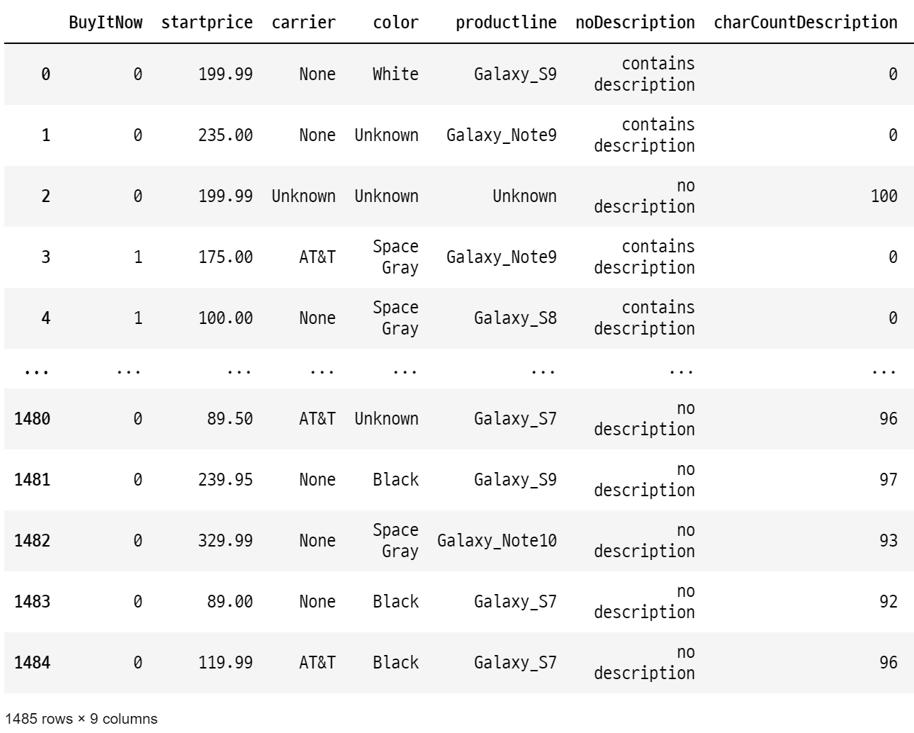
data['color'].value_counts()

>>>
Unknown       593
Black         332
White         328
Space Gray    180
Gold           52
Name: color, dtype: int64
-> color 종류가 5개로 감소되었다.
# 원 핫 인코딩을 사용해보자.
# one-hot encoding by pd.get_dummies
# ★pd.get_dummies -> 원-핫 인코딩을 해주는 함수!
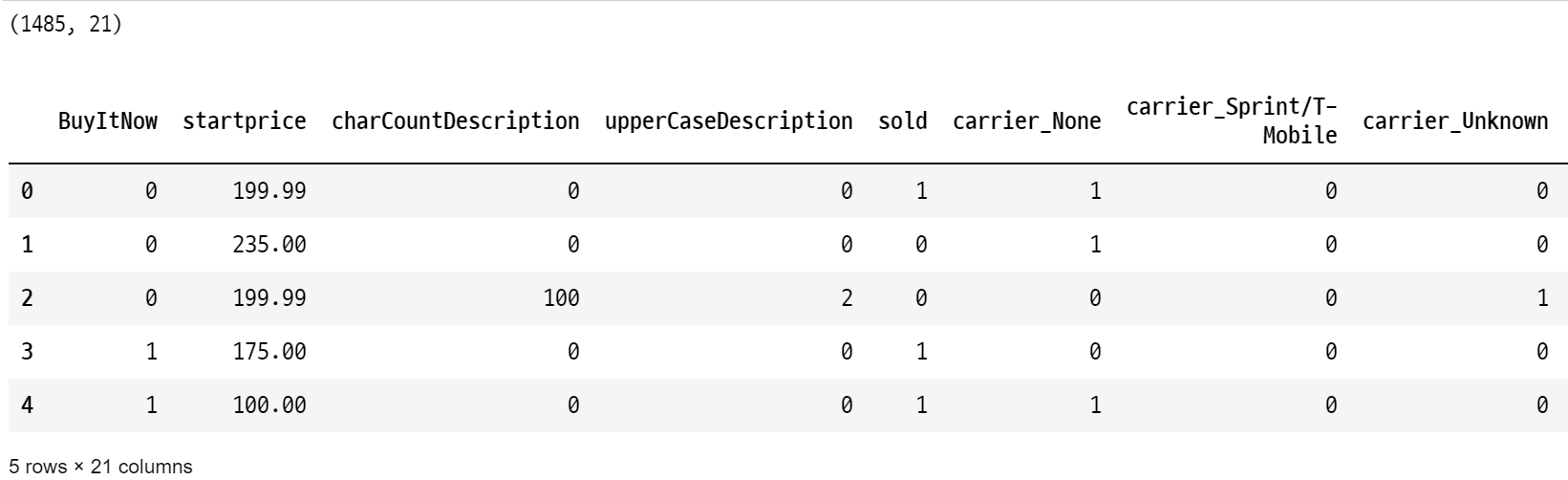
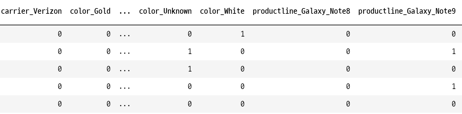
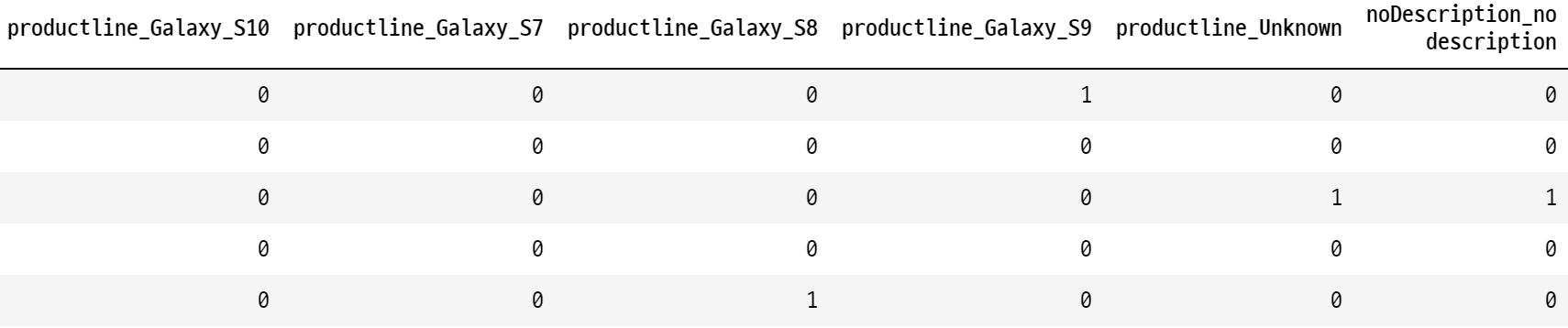
data = pd.get_dummies(data, columns = ['carrier', 'color', 'productline', 'noDescription'], drop_first=True)
# drop_first=True를 하지 않으면, 각 콜롬이 두개씩 생긴다!print(data.shape)
data.head()
data.columns

>>>
Index(['BuyItNow', 'startprice', 'charCountDescription',
       'upperCaseDescription', 'sold', 'carrier_None',
       'carrier_Sprint/T-Mobile', 'carrier_Unknown', 'carrier_Verizon',
       'color_Gold', 'color_Space Gray', 'color_Unknown', 'color_White',
       'productline_Galaxy_Note8', 'productline_Galaxy_Note9',
       'productline_Galaxy_S10', 'productline_Galaxy_S7',
       'productline_Galaxy_S8', 'productline_Galaxy_S9', 'productline_Unknown',
       'noDescription_no description'],
      dtype='object')
데이터 전처리 -> 모델링
CF)
# srtartprice를 모주 정수로 바꿔주는 함수
def float2int(x):
    return int(x)


# apply를 적용하여 startprice를 정수로 바꾸어 보자.
data['startprice'] = data['startprice'].apply(float2int)


data.info()

>>
<class 'pandas.core.frame.DataFrame'>
RangeIndex: 1485 entries, 0 to 1484
Data columns (total 21 columns):
 #   Column                        Non-Null Count  Dtype
---  ------                        --------------  -----
 0   BuyItNow                      1485 non-null   int64
 1   startprice                    1485 non-null   int64
 .
 .
 .
 .
 .
 .
 .
5 Decision Tree 모델 만들기
# 머신러닝 시 데이터 4등분해주는 함수
from sklearn.model_selection import train_test_split

data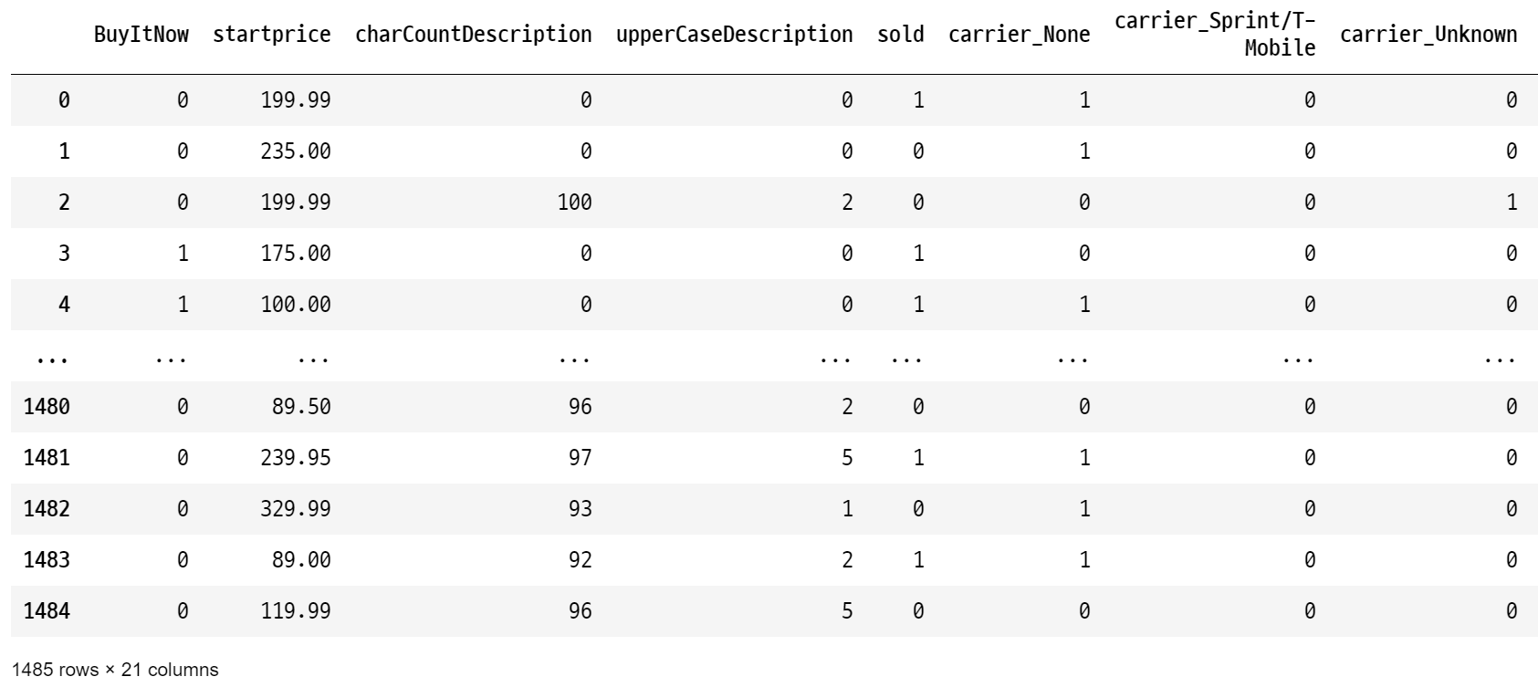
# 독립변수, 종속변수 분리
X = data.drop('sold', axis = 1)
y = data['sold']

# train, test 데이터 분리
X_train, X_test, y_train, y_test = train_test_split(X, y, test_size = 0.2, random_state=100)

from sklearn.tree import DecisionTreeClassifier

# Decision Tree 모델 생성
model = DecisionTreeClassifier(max_depth = 10)

# 모델 학습
model.fit(X_train, y_train)
6 예측
pred = model.predict(X_test)
pred

>>>
array([1, 0, 1, 1, 0, 0, 0, 1, 0, 0, 1, 0, 1, 1, 0, 1, 0, 0, 1, 1, 1, 0,
       1, 1, 0, 0, 0, 0, 0, 0, 0, 1, 0, 0, 0, 0, 0, 1, 0, 1, 0, 0, 1, 1,
       1, 1, 0, 0, 1, 0, 1, 0, 0, 1, 1, 0, 0, 1, 0, 0, 1, 0, 1, 0, 0, 1,
       1, 0, 0, 1, 0, 1, 0, 1, 1, 1, 0, 0, 1, 0, 0, 0, 0, 1, 0, 0, 0, 0,
       0, 1, 1, 0, 0, 1, 1, 0, 0, 1, 0, 1, 0, 1, 1, 0, 0, 0, 1, 0, 1, 0,
       1, 0, 0, 0, 1, 0, 0, 0, 0, 0, 1, 0, 0, 1, 0, 0, 0, 1, 0, 0, 1, 0,
       0, 1, 0, 1, 1, 0, 0, 0, 0, 1, 1, 1, 1, 0, 0, 0, 0, 1, 0, 0, 1, 0,
       0, 0, 1, 0, 0, 1, 0, 0, 0, 0, 1, 0, 0, 0, 1, 1, 1, 0, 0, 0, 1, 1,
       0, 0, 0, 1, 1, 0, 0, 0, 0, 0, 1, 0, 0, 1, 0, 0, 1, 0, 1, 0, 0, 0,
       0, 1, 0, 1, 0, 0, 0, 1, 1, 0, 1, 0, 0, 1, 1, 1, 1, 0, 0, 0, 1, 0,
       0, 0, 0, 0, 1, 0, 1, 1, 0, 1, 0, 1, 1, 1, 1, 1, 0, 1, 0, 0, 0, 1,
       1, 1, 0, 1, 0, 0, 0, 0, 0, 0, 0, 0, 0, 1, 1, 1, 0, 0, 1, 0, 1, 1,
       1, 0, 1, 0, 0, 1, 0, 1, 0, 1, 1, 1, 0, 0, 1, 1, 0, 0, 0, 1, 0, 1,
       0, 0, 0, 1, 0, 0, 0, 1, 0, 1, 1], dtype=int64)


y_test
>>>

258     1
57      0
225     1
704     0
1096    0
       ..
44      0
1399    1
1035    0
259     1
532     1
Name: sold, Length: 297, dtype: int64
7 평가
from sklearn.metrics import accuracy_score, confusion_matrix

accuracy_score(y_test, pred)
>>>
0.797979797979798
8 최적의 Max Depth 찾기 (파라미터 튜닝)
print('max_depth | accuracy')
for i in range(2, 31):
    model = DecisionTreeClassifier(max_depth = i)
    model.fit(X_train, y_train)
    pred = model.predict(X_test)
    print(i, round(accuracy_score(y_test, pred), 4))


>>>
    max_depth | accuracy
    2 0.8182
    3 0.8215
    4 0.8215
    5 0.8182
    6 0.8081
    7 0.8013
    8 0.8148
    9 0.8047
    10 0.798
    11 0.7744
    12 0.7778
    13 0.7576
    14 0.7643
    15 0.7811
    16 0.7643
    17 0.7576
    18 0.7576
    19 0.7643
    20 0.7744
    21 0.7643
    22 0.7643
    23 0.7609
    24 0.7508
    25 0.7508
    26 0.7609
    27 0.7576
    28 0.7441
    29 0.7508
    30 0.7542
8.0.0.1 위의 For loop에 숫자를 2~30까지 집어넣었으므로, score에 들어있는 숫자는 i 가 2,3,4,5,6,.. 일때 결과값.
8.0.0.2 즉, 최종적으로 얻은 score리스트에서 가장 큰 숫자가 index 1의 위치에 있다는것은 i가 3일 때를 의미함. 다시말해, i 가 3일 때 가장 높은 스코어를 보여줌
9 최적의 Max Depth를 사용하여 다시 모델링하고 평가
model = DecisionTreeClassifier(max_depth = 3)

model.fit(X_train, y_train)

pred = model.predict(X_test)

accuracy_score(y_test, pred)
>>>
0.8215488215488216

confusion_matrix(y_test, pred)
>>>
array([[148,  13],
       [ 40,  96]], dtype=int64)
10 Tree Plot 만들기
from sklearn.tree import plot_tree

len(X_train.columns)
>>> 20
# 기본 plot
plt.figure(figsize=(20, 10))

plot_tree(model);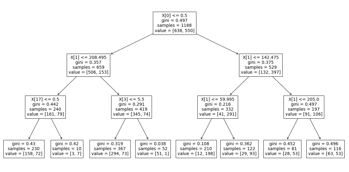
# 변수, 기준점 시각화
plt.figure(figsize=(20, 10))

plot_tree(model, feature_names=X_train.columns, fontsize=15, label ="None", max_depth = 3);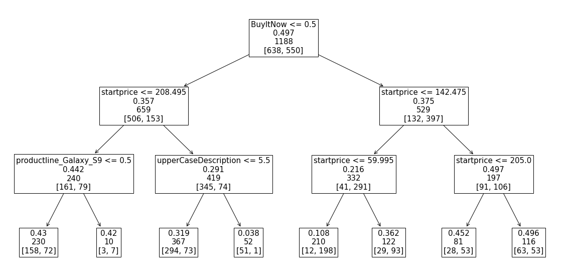
'Machine Learning > 머신러닝 완벽가이드 for Python' 카테고리의 다른 글
| ch4.10.1 스태킹 앙상블(실습) (0) | 2022.10.12 |
|---|---|
| ch. 4.10 스태킹 앙상블 모델 (0) | 2022.10.12 |
| ch4.09 분류 실습-신용카드_사기검출 (0) | 2022.10.11 |
| ch.4.09 분류 실습 2 : 신용카드 사기 예측 실습 (1) | 2022.10.11 |
| ch4.08 분류실습 _ 산탄데르 고객 만족 예측 (1) | 2022.10.11 |


