from sklearn.tree import DecisionTreeClassifier
from sklearn.datasets import load_iris
from sklearn.model_selection import train_test_split

# 워닝 무시
import warnings
warnings.filterwarnings('ignore')
1 1. iris 데이터 로드 및 분리
# 붓꽃 데이터를 로딩
iris_data = load_iris()

# 학습과 테스트 데이터 셋으로 분리
X_train , X_test , y_train , y_test = train_test_split(iris_data.data, iris_data.target,
                                                       test_size=0.2,  random_state=11)
2 2. 모델 학습(디시젼 트리)
# DecisionTree Classifier 생성
dt_clf = DecisionTreeClassifier(random_state=156)

# DecisionTreeClassifer 학습.
dt_clf.fit(X_train, y_train)
3 3. 디시젼트리 그래프비즈로 시각화
from sklearn.tree import export_graphviz

# export_graphviz()의 호출 결과로 out_file로 지정된 tree.dot 파일을 생성함.
export_graphviz(dt_clf, out_file="tree.dot", class_names=iris_data.target_names, \
                feature_names = iris_data.feature_names, impurity=True, filled=True)
import graphviz

# 위에서 생성된 tree.dot 파일을 Graphviz 읽어서 Jupyter Notebook상에서 시각화
# with open : "파일을 읽겠다"
with open("tree.dot") as f:
    dot_graph = f.read()

# graphviz.Source 메소드로 dot_graph 읽기
graph = graphviz.Source(dot_graph, format ='jpg' )
graph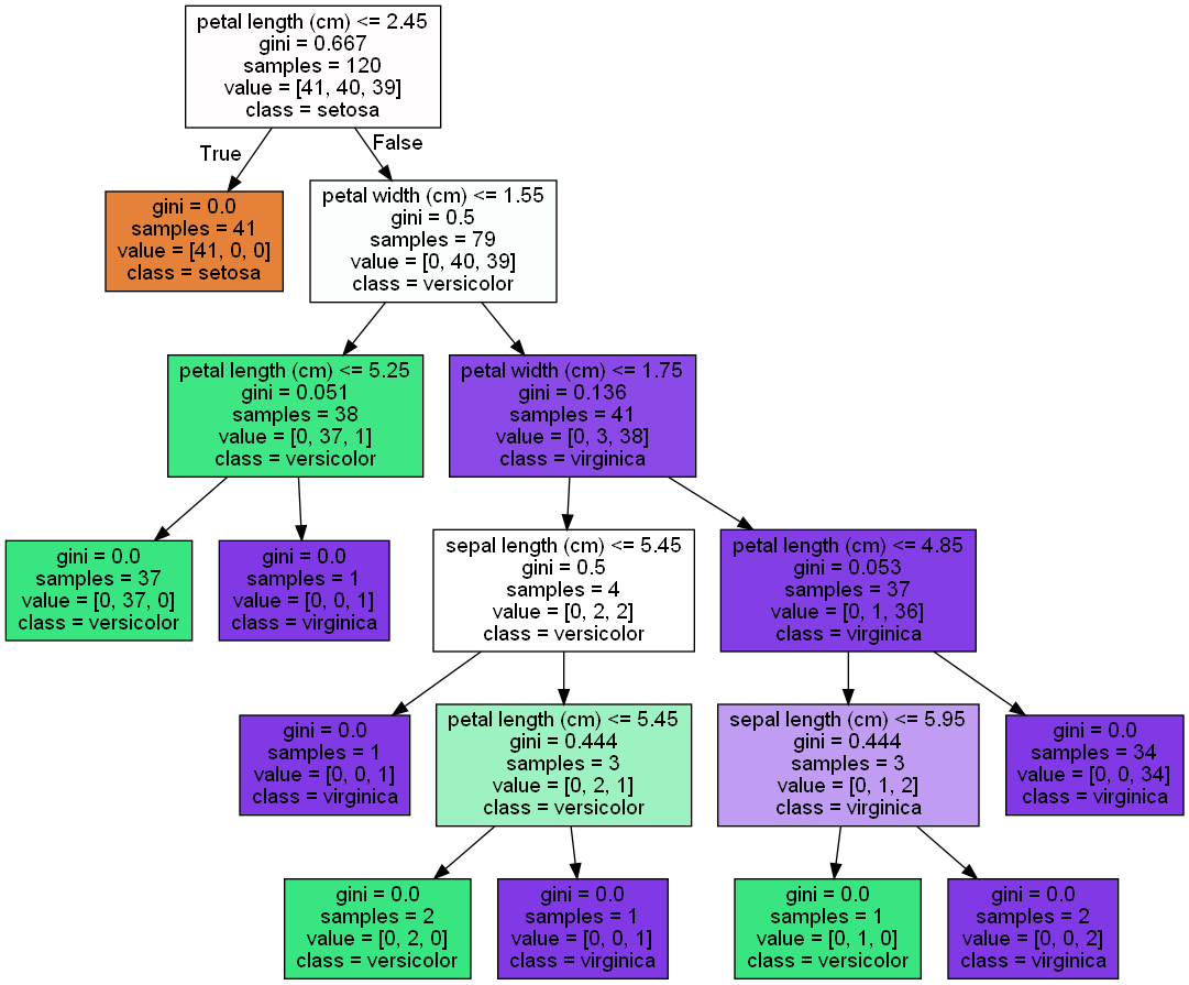
# 바탕화면에 의사결정나무 이미지 파일 저장
graph.render(filename='test_img', directory="C:/Users/JIN SEONG EUN/OneDrive/바탕 화면", format='png')
4 4. 디시젼트리의 피처 중요도 확인
import seaborn as sns
import numpy as np
%matplotlib inline
# iris 데이터의 피처 4개 확인
iris_data.feature_names
>>>
['sepal length (cm)',
'sepal width (cm)',
'petal length (cm)',
'petal width (cm)']
# 피처 4개에 대한 각각의 feature importance 확인
dt_clf.feature_importances_


# feature importance 소수 3째 자리까지
print("Feature importances:\n{0}".format(np.round(dt_clf.feature_importances_, 3)))

>>>
Feature importances:
[0.025 0.    0.555 0.42 ]
# feature별 importance 매핑
for name, value in zip(iris_data.feature_names , dt_clf.feature_importances_):
    print('{0} : {1:.3f}'.format(name, value))

# feature importance를 column 별로 시각화 하기
sns.barplot(x=dt_clf.feature_importances_ , y=iris_data.feature_names)
sepal length (cm) : 0.025
sepal width (cm) : 0.000
petal length (cm) : 0.555
petal width (cm) : 0.420
5 5. 디시젼트리 과적합(Overfitting)
from sklearn.datasets import make_classification
import matplotlib.pyplot as plt
%matplotlib inline

plt.title("3 Class values with 2 Features Sample data creation")

# 샘플 데이터 생성 : 2차원 시각화를 위해서 feature는 2개, 결정값 클래스는 3가지 유형.
X_features, y_labels = make_classification(n_features=2, n_redundant=0, n_informative=2,
                             n_classes=3, n_clusters_per_class=1, random_state=0)
X_features[:5]

>>>
array([[ 0.12041909, -1.68941375],
       [ 1.09665605,  1.79445113],
       [ 0.88426577,  1.43370121],
       [ 0.95048011, -0.56202253],
       [ 1.04421447,  0.02899023]])


y_labels[:5]

>>>
array([0, 1, 1, 1, 2])
# plot 형태로 2개의 feature로 2차원 좌표 시각화, 각 클래스값은 다른 색깔로 표시됨.
plt.scatter(X_features[:, 0], X_features[:, 1], marker='o', c=y_labels, s=25, cmap='rainbow', edgecolor='k')
import numpy as np

# Classifier의 Decision Boundary를 시각화 하는 함수
def visualize_boundary(model, X, y):
    fig,ax = plt.subplots()

    # 학습 데이타 scatter plot으로 나타내기
    ax.scatter(X[:, 0], X[:, 1], c=y, s=25, cmap='rainbow', edgecolor='k',
               clim=(y.min(), y.max()), zorder=3)
    ax.axis('tight')
    ax.axis('off')
    xlim_start , xlim_end = ax.get_xlim()
    ylim_start , ylim_end = ax.get_ylim()

    # 호출 파라미터로 들어온 training 데이타로 model 학습 .
    model.fit(X, y)
    # meshgrid 형태인 모든 좌표값으로 예측 수행.
    xx, yy = np.meshgrid(np.linspace(xlim_start, xlim_end, num=200), np.linspace(ylim_start,ylim_end, num=200))
    Z = model.predict(np.c_[xx.ravel(), yy.ravel()]).reshape(xx.shape)

    # contourf() 를 이용하여 class boundary 를 visualization 수행.
    n_classes = len(np.unique(y))
    contours = ax.contourf(xx, yy, Z, alpha=0.3,
                           levels=np.arange(n_classes + 1) - 0.5,
                           cmap='rainbow', clim=(y.min(), y.max()),
                           zorder=1)
from sklearn.tree import DecisionTreeClassifier
# 특정한 트리 생성 제약없는 결정 트리의 Decsion Boundary 시각화. -> 과적합된 모델
dt_clf = DecisionTreeClassifier().fit(X_features, y_labels)
visualize_boundary(dt_clf, X_features, y_labels)
# min_samples_leaf=6 으로 트리 생성 조건을 제약한 Decision Boundary 시각화 -> 일반화가 잘 된 모델
dt_clf = DecisionTreeClassifier( min_samples_leaf=6).fit(X_features, y_labels)
visualize_boundary(dt_clf, X_features, y_labels)
6 6. 결정 트리 실습 - Human Activity Recognition
결정 트리 실습 - 사용자 행동 인식 데이터 세트
사용자 행동 인식 네이터는 30 명에게 스마트폰 센서를 장작한 뒤
사람의 동작과 관련된 여러 가지 를 수집한 네이터입니다.
수집된 피저 세트를 기반으로 결정 트리를 이용애 어떠한 동작인지
예측해 보겠습니다.
import pandas as pd
import matplotlib.pyplot as plt
%matplotlib inline

# features.txt 파일에는 피처 이름 index와 피처명이 공백으로 분리되어 있음. 이를 DataFrame으로 로드.
feature_name_df = pd.read_csv('./human_activity/features.txt', sep='\s+',
                              header=None, names=['column_index','column_name'])

print(feature_name_df.shape)
feature_name_df.head()
# 피처명만 리스트 객체로 생성한 뒤 샘플로 10개만 추출
feature_name = feature_name_df.iloc[:, 1].values.tolist()

print('전체 피처명에서 10개만 추출:', feature_name[:10])

>>>
전체 피처명에서 10개만 추출: ['tBodyAcc-mean()-X', 'tBodyAcc-mean()-Y', 'tBodyAcc-mean()-Z',
'tBodyAcc-std()-X', 'tBodyAcc-std()-Y', 'tBodyAcc-std()-Z', 'tBodyAcc-mad()-X', 'tBodyAcc-mad()-Y', 'tBodyAcc-mad()-Z', 'tBodyAcc-max()-X']
**중복 feature명에 대해서 원본 feature 명에 '_1(또는2)'를 추가로 부여하는 함수인 get_new_feature_name_df() 생성**
def get_new_feature_name_df(old_feature_name_df):
    feature_dup_df = pd.DataFrame(data=old_feature_name_df.groupby('column_name').cumcount(), columns=['dup_cnt'])
    feature_dup_df = feature_dup_df.reset_index()
    new_feature_name_df = pd.merge(old_feature_name_df.reset_index(), feature_dup_df, how='outer')
    new_feature_name_df['column_name'] = new_feature_name_df[['column_name', 'dup_cnt']].apply(lambda x : x[0]+'_'+str(x[1])
                                                                                           if x[1] >0 else x[0] ,  axis=1)
    new_feature_name_df = new_feature_name_df.drop(['index'], axis=1)
    return new_feature_name_df


pd.options.display.max_rows = 999
new_feature_name_df = get_new_feature_name_df(feature_name_df)
new_feature_name_df[new_feature_name_df['dup_cnt'] > 0]
# 피처명만 리스트 객체로 생성한 뒤 샘플로 10개만 추출
feature_name = feature_name_df.iloc[:, 1].values.tolist()

print('전체 피처명에서 10개만 추출:', feature_name[:10])

>>>
전체 피처명에서 10개만 추출: ['tBodyAcc-mean()-X', 'tBodyAcc-mean()-Y', 'tBodyAcc-mean()-Z', 'tBodyAcc-std()-X', 'tBodyAcc-std()-Y', 'tBodyAcc-std()-Z', 'tBodyAcc-mad()-X', 'tBodyAcc-mad()-Y', 'tBodyAcc-mad()-Z', 'tBodyAcc-max()-X']
**중복 feature명에 대해서 원본 feature 명에 '_1(또는2)'를 추가로 부여하는 함수인 get_new_feature_name_df() 생성**
def get_new_feature_name_df(old_feature_name_df):
    feature_dup_df = pd.DataFrame(data=old_feature_name_df.groupby('column_name').cumcount(), columns=['dup_cnt'])
    feature_dup_df = feature_dup_df.reset_index()
    new_feature_name_df = pd.merge(old_feature_name_df.reset_index(), feature_dup_df, how='outer')
    new_feature_name_df['column_name'] = new_feature_name_df[['column_name', 'dup_cnt']].apply(lambda x : x[0]+'_'+str(x[1])
                                                                                           if x[1] >0 else x[0] ,  axis=1)
    new_feature_name_df = new_feature_name_df.drop(['index'], axis=1)
    return new_feature_name_df
pd.options.display.max_rows = 999
new_feature_name_df = get_new_feature_name_df(feature_name_df)
new_feature_name_df[new_feature_name_df['dup_cnt'] > 0]
import pandas as pd

# train, test 데이터 분리해주는 함수
def get_human_dataset( ):

    # 각 데이터 파일들은 공백으로 분리되어 있으므로 read_csv에서 공백 문자를 sep으로 할당.
    feature_name_df = pd.read_csv("C:/Users/JIN SEONG EUN/OneDrive/바탕 화면/빅데이터 분석가 과정/머신러닝/실강/CH04/UCI HAR Dataset/features.txt",sep='\s+',
                      header=None,names=['column_index','column_name'])

    # 중복된 feature명을 새롭게 수정하는 get_new_feature_name_df()를 이용하여 새로운 feature명 DataFrame생성.
    new_feature_name_df = get_new_feature_name_df(feature_name_df)

    # DataFrame에 피처명을 컬럼으로 부여하기 위해 리스트 객체로 다시 변환
    feature_name = new_feature_name_df.iloc[:, 1].values.tolist()

    # 학습 피처 데이터 셋과 테스트 피처 데이터을 DataFrame으로 로딩. 컬럼명은 feature_name 적용
    X_train = pd.read_csv("./UCI HAR Dataset/train/X_train.txt",sep='\s+', names=feature_name )
    X_test = pd.read_csv('./UCI HAR Dataset/test/X_test.txt',sep='\s+', names=feature_name)

    # 학습 레이블과 테스트 레이블 데이터을 DataFrame으로 로딩하고 컬럼명은 action으로 부여
    y_train = pd.read_csv('./UCI HAR Dataset/train/y_train.txt',sep='\s+',header=None,names=['action'])
    y_test = pd.read_csv('./UCI HAR Dataset/test/y_test.txt',sep='\s+',header=None,names=['action'])

    # 로드된 학습/테스트용 DataFrame을 모두 반환
    return X_train, X_test, y_train, y_test


X_train, X_test, y_train, y_test = get_human_dataset()
print(X_train.shape, '\n')
print(X_train.info())

>>>

(7352, 561)

<class 'pandas.core.frame.DataFrame'>
RangeIndex: 7352 entries, 0 to 7351
Columns: 561 entries, tBodyAcc-mean()-X to angle(Z,gravityMean)
dtypes: float64(561)
memory usage: 31.5 MB
None
print(y_train['action'].value_counts())

>>>
6    1407
5    1374
4    1286
1    1226
2    1073
3     986
Name: action, dtype: int64
# 데이터에 null값은 없다.
X_train.isnull().sum().sum()
>>> 0
from sklearn.tree import DecisionTreeClassifier
from sklearn.metrics import accuracy_score

# DecisionTreeClassifier 클래스 객체 생성
dt_clf = DecisionTreeClassifier(random_state=156)

# 학습
dt_clf.fit(X_train , y_train)

# 예측
pred = dt_clf.predict(X_test)

# 평가 - 정확도 확인
accuracy = accuracy_score(y_test, pred)
print('결정 트리 예측 정확도: {0:.4f}'.format(accuracy), '\n')

# DecisionTreeClassifier의 하이퍼 파라미터 추출
print('DecisionTreeClassifier 기본 하이퍼 파라미터:\n', dt_clf.get_params())

>>>
결정 트리 예측 정확도: 0.8548

DecisionTreeClassifier 기본 하이퍼 파라미터:
 {'ccp_alpha': 0.0, 'class_weight': None, 'criterion': 'gini', 'max_depth': None, 'max_features': None, 'max_leaf_nodes': None, 'min_impurity_decrease': 0.0, 'min_samples_leaf': 1, 'min_samples_split': 2, 'min_weight_fraction_leaf': 0.0, 'random_state': 156, 'splitter': 'best'}
-> GridSearchCV를 적용하기 전 모델의 정확도는 0.85
GridSearchCV를 적용해서 하이퍼 파라미터 튜닝을 하면 정확도가 올라갈까?
7 GridSearchCV로 DecisionTreeClassifier 하이퍼 파라미터 튜닝
%%time
# 수행시간 1~2분
from sklearn.model_selection import GridSearchCV

params = {
    'max_depth' : [6, 8 ,10, 12, 16 ,20, 24]
}

grid_cv = GridSearchCV(dt_clf, param_grid=params, scoring='accuracy', cv=5, verbose=1)
grid_cv.fit(X_train , y_train)
print('GridSearchCV 최고 평균 정확도 수치:{0:.4f}'.format(grid_cv.best_score_))
print('GridSearchCV 최적 하이퍼 파라미터:', grid_cv.best_params_)


>>>

Fitting 5 folds for each of 7 candidates, totalling 35 fits
GridSearchCV 최고 평균 정확도 수치:0.8513
GridSearchCV 최적 하이퍼 파라미터: {'max_depth': 16}
CPU times: user 1min 22s, sys: 324 ms, total: 1min 22s
Wall time: 1min 23s
# GridSearchCV객체의 cv_results_ 속성을 DataFrame으로 생성.
cv_results_df = pd.DataFrame(grid_cv.cv_results_)
cv_results_df.columns

>>>
Index(['mean_fit_time', 'std_fit_time', 'mean_score_time', 'std_score_time',
       'param_max_depth', 'params', 'split0_test_score', 'split1_test_score',
       'split2_test_score', 'split3_test_score', 'split4_test_score',
       'mean_test_score', 'std_test_score', 'rank_test_score'],
      dtype='object')
# max_depth 파라미터 값과 그때의 테스트(Evaluation)셋, 학습 데이터 셋의 정확도 수치 추출
# 사이킷런 버전이 업그레이드 되면서 아래의 GridSearchCV 객체의 cv_results_에서 mean_train_score는 더이상 제공되지 않습니다
# cv_results_df[['param_max_depth', 'mean_test_score', 'mean_train_score']]

# max_depth 파라미터 값과 그때의 테스트(Evaluation)셋, 학습 데이터 셋의 정확도 수치 추출
result_rank = cv_results_df[['param_max_depth', 'mean_test_score', 'rank_test_score']]   # 리스트에서 'mean_train_score' 제거한 상태

# test socre 순위 기준으로 정렬해보면 아래와 같다.
result_rank.sort_values(by='rank_test_score')
-> 위에서는 검증 데이터셋으로 성능을 측정해본 것이고
이제 테스트 데이터로 성능을 측정해보자
# max_depth 값을 변화 시키면서 그때마다 학습과 테스트 셋에서의 예측 성능 측정
max_depths = [ 6, 8 ,10, 12, 16 ,20, 24]

for depth in max_depths:
    dt_clf = DecisionTreeClassifier(max_depth=depth, random_state=156)
    dt_clf.fit(X_train , y_train)
    pred = dt_clf.predict(X_test)
    accuracy = accuracy_score(y_test , pred)
    print('max_depth = {0} 정확도: {1:.4f}'.format(depth , accuracy))


>>>
max_depth = 6 정확도: 0.8558
max_depth = 8 정확도: 0.8707
max_depth = 10 정확도: 0.8673
max_depth = 12 정확도: 0.8646
max_depth = 16 정확도: 0.8575
max_depth = 20 정확도: 0.8548
max_depth = 24 정확도: 0.8548
-> 모델을 테스트셋에 적용해본 결과 max_depth가 8인 경우 가장 성능이 좋다.
%%time
# min_samples_split 하이퍼 파라미터도 추가해서 GridSearchCV 수행 (수행시간 1~2분 정도)
params = {
    'max_depth' : [ 8 , 12, 16 , 20 ],
    'min_samples_split' : [ 16, 24 ],
}

grid_cv = GridSearchCV(dt_clf, param_grid=params, scoring='accuracy', cv=5, verbose=1 )

grid_cv.fit(X_train , y_train)
print('GridSearchCV 최고 평균 정확도 수치: {0:.4f}'.format(grid_cv.best_score_), '\n')
print('GridSearchCV 최적 하이퍼 파라미터:', grid_cv.best_params_)

>>>
Fitting 5 folds for each of 8 candidates, totalling 40 fits
GridSearchCV 최고 평균 정확도 수치: 0.8549

GridSearchCV 최적 하이퍼 파라미터: {'max_depth': 8, 'min_samples_split': 16}
CPU times: user 1min 36s, sys: 388 ms, total: 1min 37s
Wall time: 1min 37s
-> 그리드서치로 찾아진 최적의 하이퍼 파라미터를 가진 모델을 가지고 테스트 데이터에 적용해보자.
best_df_clf = grid_cv.best_estimator_

pred1 = best_df_clf.predict(X_test)
accuracy = accuracy_score(y_test , pred1)
print('결정 트리 예측 정확도:{0:.4f}'.format(accuracy))

>>>
결정 트리 예측 정확도:0.8717
-> 결론 : 그리드서치로 하이퍼 파라미터 튜닝을 했더니 기존의 정확도가 0.85에서 0.87로 상승했음을 볼 수 있다..
# 피처 중요도 확인해보기
import seaborn as sns

ftr_importances_values = best_df_clf.feature_importances_
ftr_importances_values

>>>
array([0.        , 0.        , 0.        , 0.        , 0.00175182,
       0.        , 0.        , 0.        , 0.        , 0.00217984,
       0.        , 0.        , 0.        , 0.        , 0.        ,
       0.        , 0.        , 0.        , 0.        , 0.        ,
       0.        , 0.        , 0.        , 0.        , 0.        ,
       0.        , 0.        , 0.        , 0.00034009, 0.        ,
       0.        , 0.        , 0.        , 0.        , 0.        ,
       0.        , 0.        , 0.00997154, 0.        , 0.        ,
       0.        , 0.        , 0.        , 0.        , 0.        ,
       0.        , 0.        , 0.        , 0.        , 0.00122902,
       0.00629033, 0.        , 0.2533544 , 0.002077  , 0.00291231,
       0.        , 0.        , 0.02047009, 0.        , 0.        ,
       0.        , 0.        , 0.        , 0.        , 0.        ,
       0.        , 0.        , 0.0024461 , 0.        , 0.        ,
       0.        , 0.00302454, 0.        , 0.        , 0.10188539,
       0.        , 0.        , 0.        , 0.        , 0.        ,
       0.        , 0.        , 0.        , 0.        , 0.        ,
       0.        , 0.        , 0.        , 0.        , 0.00124463,
       0.        , 0.        , 0.        , 0.        , 0.        ,
       0.        , 0.        , 0.        , 0.        , 0.        ,
       0.        , 0.0011924 , 0.        , 0.        , 0.        ,
       0.        , 0.        , 0.00065083, 0.        , 0.        ,
       0.        , 0.00034211, 0.        , 0.        , 0.        ,
       0.        , 0.        , 0.00396674, 0.        , 0.        ,
       0.        , 0.        , 0.        , 0.        , 0.        ,
       0.        , 0.        , 0.        , 0.        , 0.00854963,
       0.        , 0.        , 0.00437287, 0.        , 0.        ,
       0.        , 0.        , 0.        , 0.        , 0.00264146,
       0.        , 0.        , 0.        , 0.        , 0.        ,
       0.        , 0.        , 0.        , 0.        , 0.0005292 ,
       0.        , 0.        , 0.        , 0.        , 0.        ,
       0.        , 0.        , 0.00233647, 0.        , 0.01651344,
       0.        , 0.        , 0.        , 0.        , 0.        ,
       0.        , 0.00033559, 0.        , 0.        , 0.0034711 ,
       0.        , 0.        , 0.        , 0.        , 0.        ,
       0.        , 0.        , 0.        , 0.00124472, 0.        ,
       0.        , 0.        , 0.        , 0.        , 0.        ,
       0.        , 0.        , 0.        , 0.        , 0.        ,
       0.        , 0.        , 0.        , 0.        , 0.        ,
       0.        , 0.0003379 , 0.        , 0.        , 0.        ,
       0.        , 0.        , 0.        , 0.        , 0.        ,
       0.        , 0.        , 0.        , 0.        , 0.        ,
       0.        , 0.        , 0.        , 0.        , 0.        ,
       0.        , 0.        , 0.        , 0.        , 0.        ,
       0.        , 0.        , 0.01574123, 0.        , 0.        ,
       0.        , 0.        , 0.        , 0.        , 0.        ,
       0.        , 0.        , 0.        , 0.        , 0.        ,
       0.        , 0.        , 0.        , 0.        , 0.        ,
       0.        , 0.        , 0.        , 0.        , 0.        ,
       0.        , 0.        , 0.        , 0.        , 0.        ,
       0.        , 0.        , 0.        , 0.        , 0.        ,
       0.        , 0.        , 0.        , 0.        , 0.        ,
       0.        , 0.        , 0.        , 0.00041491, 0.        ,
       0.        , 0.        , 0.        , 0.        , 0.        ,
       0.        , 0.        , 0.        , 0.        , 0.        ,
       0.00882456, 0.        , 0.        , 0.        , 0.        ,
       0.        , 0.        , 0.        , 0.        , 0.        ,
       0.        , 0.        , 0.        , 0.        , 0.        ,
       0.        , 0.        , 0.        , 0.        , 0.        ,
       0.        , 0.        , 0.        , 0.        , 0.        ,
       0.        , 0.        , 0.00233064, 0.        , 0.        ,
       0.        , 0.        , 0.        , 0.        , 0.        ,
       0.        , 0.        , 0.        , 0.        , 0.        ,
       0.        , 0.        , 0.        , 0.        , 0.        ,
       0.        , 0.        , 0.        , 0.        , 0.        ,
       0.        , 0.        , 0.        , 0.        , 0.        ,
       0.        , 0.        , 0.        , 0.        , 0.        ,
       0.        , 0.        , 0.        , 0.        , 0.        ,
       0.        , 0.        , 0.        , 0.        , 0.        ,
       0.        , 0.        , 0.        , 0.        , 0.        ,
       0.        , 0.        , 0.        , 0.        , 0.        ,
       0.        , 0.        , 0.        , 0.        , 0.        ,
       0.        , 0.        , 0.        , 0.        , 0.        ,
       0.        , 0.        , 0.        , 0.        , 0.        ,
       0.        , 0.        , 0.        , 0.        , 0.        ,
       0.        , 0.        , 0.        , 0.        , 0.        ,
       0.        , 0.        , 0.        , 0.00066434, 0.        ,
       0.        , 0.        , 0.        , 0.        , 0.21258352,
       0.        , 0.        , 0.        , 0.00145481, 0.        ,
       0.        , 0.        , 0.        , 0.        , 0.        ,
       0.        , 0.        , 0.        , 0.        , 0.        ,
       0.        , 0.        , 0.        , 0.        , 0.00142006,
       0.        , 0.        , 0.        , 0.        , 0.        ,
       0.        , 0.        , 0.        , 0.00220174, 0.        ,
       0.00118853, 0.        , 0.        , 0.        , 0.        ,
       0.0017426 , 0.        , 0.        , 0.        , 0.        ,
       0.        , 0.        , 0.00524676, 0.        , 0.        ,
       0.        , 0.        , 0.        , 0.        , 0.        ,
       0.        , 0.        , 0.        , 0.00283466, 0.        ,
       0.        , 0.        , 0.        , 0.02397088, 0.        ,
       0.        , 0.        , 0.        , 0.        , 0.        ,
       0.        , 0.        , 0.        , 0.        , 0.        ,
       0.        , 0.        , 0.        , 0.        , 0.        ,
       0.        , 0.        , 0.        , 0.        , 0.        ,
       0.        , 0.        , 0.        , 0.        , 0.        ,
       0.        , 0.        , 0.        , 0.        , 0.        ,
       0.        , 0.        , 0.        , 0.        , 0.        ,
       0.        , 0.        , 0.        , 0.        , 0.        ,
       0.        , 0.        , 0.        , 0.        , 0.        ,
       0.        , 0.        , 0.        , 0.        , 0.        ,
       0.        , 0.        , 0.        , 0.00259031, 0.        ,
       0.        , 0.        , 0.        , 0.11547846, 0.        ,
       0.        , 0.        , 0.        , 0.        , 0.        ,
       0.        , 0.        , 0.        , 0.        , 0.        ,
       0.        , 0.        , 0.        , 0.        , 0.        ,
       0.        , 0.        , 0.        , 0.        , 0.        ,
       0.        , 0.        , 0.        , 0.        , 0.        ,
       0.        , 0.        , 0.        , 0.00138302, 0.        ,
       0.        , 0.        , 0.        , 0.        , 0.        ,
       0.        , 0.        , 0.        , 0.        , 0.        ,
       0.        , 0.        , 0.        , 0.        , 0.        ,
       0.        , 0.00129082, 0.        , 0.00098939, 0.1390006 ,
       0.00298663])
# Top 중요도로 정렬을 쉽게 하고, 시본(Seaborn)의 막대그래프로 쉽게 표현하기 위해 Series변환
ftr_importances = pd.Series(ftr_importances_values, index=X_train.columns)

# 중요도값 순으로 Series를 정렬. 피처는 중요도 상위 20개만 추출해서 정렬.
ftr_top20 = ftr_importances.sort_values(ascending=False)[:20]

plt.figure(figsize=(8, 6))
plt.title('Feature importances Top 20')
sns.barplot(x=ftr_top20 , y = ftr_top20.index)
plt.show()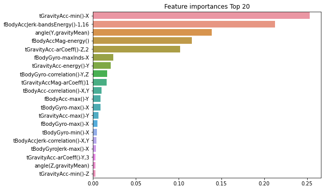
# 피처 20개 이름
ftr_top20.index

>>>
Index(['tGravityAcc-min()-X', 'fBodyAccJerk-bandsEnergy()-1,16',
       'angle(Y,gravityMean)', 'fBodyAccMag-energy()',
       'tGravityAcc-arCoeff()-Z,2', 'fBodyGyro-maxInds-X',
       'tGravityAcc-energy()-Y', 'tBodyGyro-correlation()-Y,Z',
       'tGravityAccMag-arCoeff()1', 'tBodyAcc-correlation()-X,Y',
       'fBodyAcc-max()-Y', 'tBodyGyro-max()-X', 'tGravityAcc-max()-Y',
       'fBodyGyro-max()-X', 'tBodyGyro-min()-X',
       'tBodyAccJerk-correlation()-X,Y', 'tBodyGyroJerk-max()-X',
       'tGravityAcc-arCoeff()-Y,3', 'angle(Z,gravityMean)',
       'tGravityAcc-min()-Z'],
dtype='object')'Machine Learning > 머신러닝 완벽가이드 for Python' 카테고리의 다른 글
| ch.4.4 앙상블 - 배깅 (1) | 2022.10.06 |
|---|---|
| ch.4.3 앙상블 - 보팅 (1) | 2022.10.06 |
| ch.4.1~2. 분류의 종류, 결정 트리 (1) | 2022.10.06 |
| ch03 요약 (0) | 2022.10.06 |
| ch.3.6 실습 파마 인디언 당뇨병 예측(실습) (0) | 2022.10.06 |


